Code

# Load packages
library(tmap)
library(sp)
library(spData)
library(sf)
library(tidyverse)
library(lubridate)
library(lfe)
library(patchwork)
library(gtsummary)
library(gt)
library(sjPlot)
library(knitr)

Code

#read in data. I downloaded three csv files from MARINe: two photo plots of motile inverts and one percent cover. I went with the raw data for all files. 
data_dir <- "/Users/jfrench/Documents/MEDS/eds-222/final_project/data"

# Read in wrangled data that includes invert data with drought conditions and sst.
invert_data <- readRDS(file.path(data_dir, "shannon_lag_sst.RDS")) |> 
  mutate("sample_year" = as.character(sample_year)) |>
  mutate("sample_year" = paste0(sample_year, "-01-01")) |> 
  mutate("sample_year" = lubridate::ymd(sample_year)) |> 
  filter(intertidal_sitename != "Cape Arago")

Code

# Read in the shape file
ecoregions_shape <- read_sf(dsn = file.path(data_dir,"/epa_ecoareas/NA_CEC_Eco_Level3.shp"),
                      layer = "NA_CEC_Eco_Level3") |> 
  st_transform("EPSG:4955")

# Limiting to the Marine West Coast Forest Ecoregion, level 3
# Add buffer to capture sites that are a little too far seaward to fall within the ecoregion polygon. 
ecoregion <- ecoregions_shape |> 
  dplyr::filter(NA_L3CODE == "7.1.8") |> 
  st_buffer(25) |> 
  st_transform("EPSG:4955")

west_coast <- us_states |> 
  filter(NAME %in% c("Washington", "Oregon", "California"))

Introduction

The rocky intertidal zone is one of the most complex and challenging ecosystems in the world ^1,2,4. Within a single tidal cycle, organisms are exposed to a wide range of environmental extremes. During high tide organisms experience crashing waves and debris that can dislodge or crush them, while low tide brings the risk of extreme heat and desiccation ^1,2,4,5. Predation, competition, oceanographic conditions, and resource availability are ever present and add to the already overwhelming complexity of this habitat ^1,2,6. With so much going on in such a small area the rocky intertidal zone has been used as a natural laboratory for ecologists seeking to understand species interactions and responses to environmental extremes ². An enormous amount of research has been conducted in rocky intertidal zones all over the world but noticeably absent from this body of work is how drought might impact intertidal organisms ⁷.

With climate change and changing patterns of precipitation, droughts are expected to occur more frequently and with greater severity and duration ⁸. Drought has been shown to impact species abundance and composition in freshwater stream invertebrate communities through reduction in pool connectivity and increasing predation ⁹. In the rocky intertidal zone reduction in terrestrial organic matter (TOM) is a more likely cause of reduced abundance and diversity during drought. Small streams that drain directly into the ocean transport TOM in the form of leaf litter that is consumed by motile invertebrate grazers in the intertidal ¹⁰. Food availability throughout the year can have major impacts on reproductive output, larvae survival, and recruitment ^10,11. This is why I hypothesize that drought will negatively impact abundance and diversity of motile invertebrates in the rocky intertidal zone in the Coast Range Ecoregion of California (Fig 1).

Code

# set tmap to interactive
tmap_mode(mode = "view")

Code

# Create ecoregion and site map
eco_site_map <- 
  tm_shape(ecoregion) + 
  tm_borders(col = "purple4") +
  tm_shape(invert_data) +
  tm_dots(col = 'intertidal_sitename', 
          title = 'Sites', 
          palette = "RdPu",
          size = 0.1) 
                
eco_site_map

_{Fig. 1 Map showing the site locations and extent of the Coast Range Ecoregion.}

Data Description

To test my hypothesis, I used motile invertebrate count data from Multi-Agency Rocky Intertidal Network through UC Santa Cruz and drought impact data from U.S. Drought Monitor produced by a partnership between the National Drought Mitigation Center (NDMC) at the University of Nebraska-Lincoln, the National Oceanic and Atmospheric Administration (NOAA), and the U.S. Department of Agriculture (USDA) ¹².

The motile invertebrate count data was the result of long-term monitoring efforts from multiple agencies and includes counts of species from 1999 to 2019 at intertidal sites along the West Coast of The United States ¹³. Observations were made in summer (June-September), fall (October-January), or spring (February-May) ¹⁴. For this analysis, only observations from spring and fall were considered in an attempt to limit the affect of extreme heat as a confounding variable. To ensure similarity in climate and broad scale ecological factors only sites in the Coast Range level III ecoregion, defined by the EPA, were included ¹⁵.

The drought impact data were in the form of polygons indicating the level of drought impact in that area. Drought impact levels are determined from a range of drought indices and range from D0-Abnormally dry to D4-Exceptional drought. More information about how these levels are determined can be found on U.S. Drought Monitor’s website. Drought condition for each observation was determined by finding the drought polygons that each site fell into spatially and temporally overlapped with the observation. Because the temporal resolution of the invertebrate counts is four months each observation potentially fell into multiple polygons, the most severe drought condition was chosen as the drought condition for the observation.

Analysis

To determine if drought has an impact on the abundance and diversity of motile intertidal invertebrates I combined the drought impact data with the motile invertebrate count data, as described above. I then summed the mean number of invertebrates per plot for each site and year. I then calculated the Shannon diversity index at each site for each year. After this aggregation I defined each observation as either the total mean number of organisms per site per year or the Shannon diversity index per site per year (Equation 1).

\[H’ = -\sum_{i=1}^s p_i \log(p_i)\] _Equation ₁

I simplified the drought impacts variable to a binary of “Drought” or “No Drought”. If a site experienced any drought impacts as described by the U.S. Drought Monitor in the observation year, I assigned it drought for the entire year, if no drought impacts were recorded I assigned no drought. This simplification allowed for easier comparison between sites as not all sites experienced all drought conditions in all years. Additionally, I generated autocorrelation plots of abundance (mean number of organisms per plot) and Shannon diversity index to confirm correlation between either variable and its value the previous year (Fig 2).

I then fit fixed effects linear models, using the felm() function from the lfe package, that regressed drought condition in the current year on Shannon diversity index and abundance. I repeated this process for regressing the previous years drought condition on Shannon diversity index and abundance. The fixed effect model allowed each site to be held constant such that any results would not be the result of inherent differences in diversity and abundance between sites.

Results

The autocorrelation plots showed a significant correlation between both abundance and Shannon diversity index in the current year and their value the following year. This gave me confidence in incorporating the prior year drought condition in the following models.

Code

par(mfrow=c(1,2))
# autocorrelation plot 
abundance_acf <- acf(invert_data$mean_org_per_plot, 
                     lag.max = 18, 
                     main = "Abundance")
graphics::mtext("Fig. 2 Autocorrelation plots, each lag represents one year.", side = 1, 
                line = 4,
                adj = 0)
shannon_acf <- acf(invert_data$shannon_index, 
                   lag.max = 18, 
                   main = "Shannon Index",
                   axes = FALSE,
                   ylab = "") 
axis(1)
box(col ="black")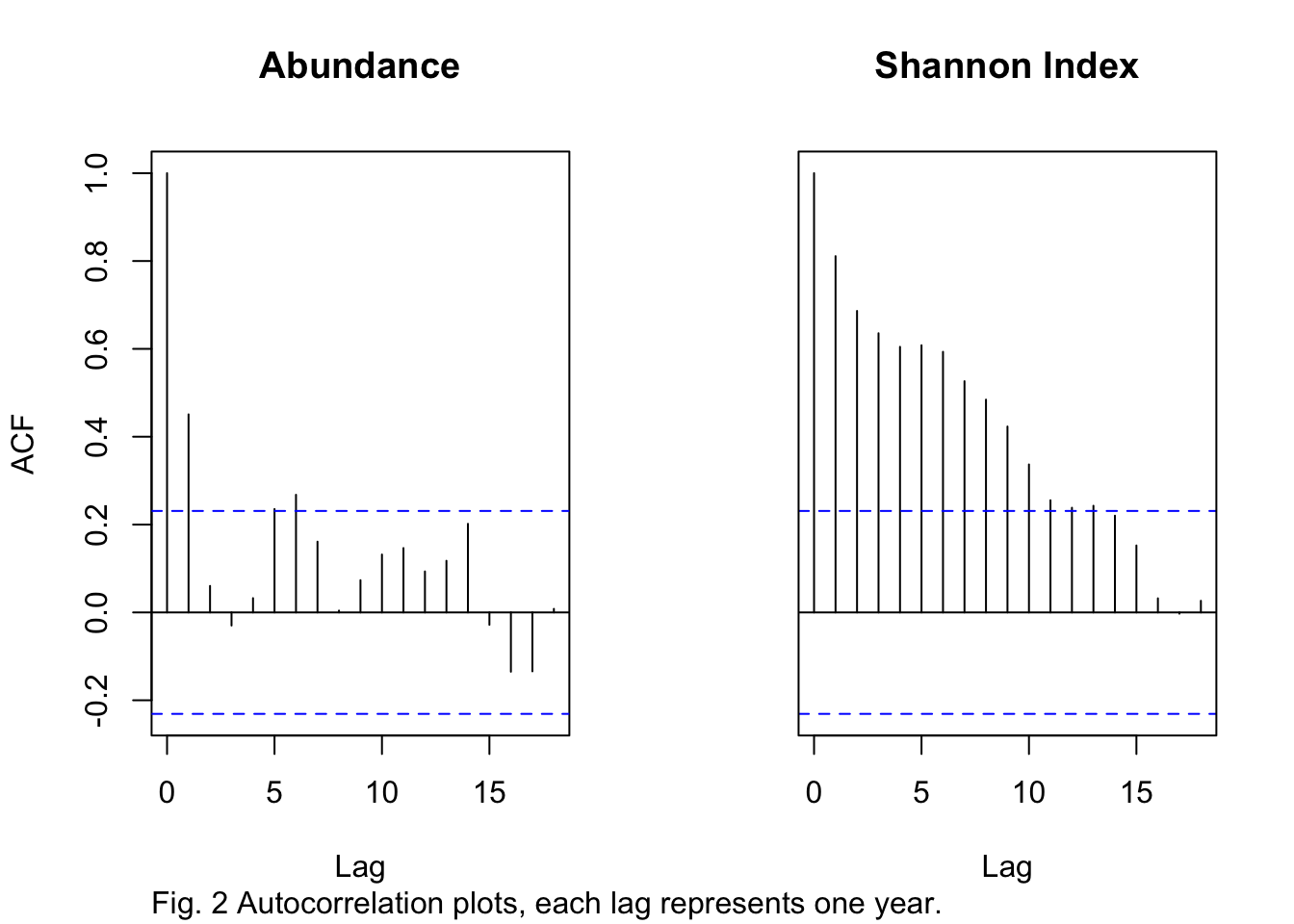

Drought condition in the year observations were made had a marginally significant effect on Shannon diversity index (p-value = 0.074) and no significant impact on abundance. The model predicts that a site not experiencing drought will have a 0.06 reduction in Shannon diversity index compared to the sites baseline. Drought condition in the year before observations were made did not have a significant impact on either Shannon diversity index or abundance.

A summary of all model outputs can be found in tables 1 and 2 below. Residuals and Q-Q plots assessing the the model regressing current year drought on Shannon diversity index can be found under supplemental figures.

Code

# fit models
## Models of current year drought impact on Shannon divversity index and abundance
shannon_model <- felm(shannon_index~ drought_simple | intertidal_sitename, data = invert_data)
shannon_mod_sum <- summary(shannon_model)

abundance_model <- felm(mean_org_per_plot~drought_simple | intertidal_sitename, data = invert_data)
abundance_mod_sum <- summary(abundance_model)

## Models of prior year drought impact on Shannon diversity index and abundance.
shannon_lag_model <- felm(shannon_index ~ drought_lag_simple | intertidal_sitename, data = invert_data)
shannon_lag_mod_sum <- summary(shannon_lag_model)

abundance_lag_model <- felm(mean_org_per_plot~drought_lag_simple | intertidal_sitename, data = invert_data)
abundance_lag_mod_sum <- summary(abundance_lag_model)

Code

# Create summary tables of both sets of models from above
shannon_mod_tbl <- tbl_regression(shannon_model,
                                  label = c(drought_simple ~ "Drought Condition")) |> 
  modify_caption("Table 1. Current Year Drought Impact Model Summary") 

abundance_mod_tbl <- tbl_regression(abundance_model,
                                    label = c(drought_simple ~ "Drought Condition"))  
current_year_list <- list(shannon_mod_tbl, 
                          abundance_mod_tbl)
current_year_summary <- tbl_merge(current_year_list, 
                                  tab_spanner = c("Shannon diversity index", 
                                                  "Abundance")) 


shannon_lag_mod_tbl <- tbl_regression(shannon_lag_model,
                                      label = c(drought_lag_simple ~ "Drought Condition")) |> 
  modify_caption("Table 2. Prior Year Drought Impact Model Summary")


abundance_lag_mod_tbl <- tbl_regression(abundance_lag_model,
                                        label = c(drought_lag_simple ~ "Drought Condition")) 
lag_list <- list(shannon_lag_mod_tbl, 
                 abundance_lag_mod_tbl)

lag_year_summary <- tbl_merge(lag_list, 
                              tab_spanner = c("Shannon diversity index", 
                                              "Abundance"))


current_year_summary

Table 1. Current Year Drought Impact Model Summary
Characteristic	Shannon diversity index			Abundance
Characteristic	Beta	95% CI¹	p-value	Beta	95% CI¹	p-value
Drought Condition
drought	—	—		—	—
no_drought	-0.06	-0.12, 0.01	0.074	59	-552, 670	0.8
¹ CI = Confidence Interval

Code

lag_year_summary

Table 2. Prior Year Drought Impact Model Summary
Characteristic	Shannon diversity index			Abundance
Characteristic	Beta	95% CI¹	p-value	Beta	95% CI¹	p-value
Drought Condition
drought	—	—		—	—
no_drought	-0.01	-0.08, 0.06	0.7	526	-109, 1,162	0.10
¹ CI = Confidence Interval

Discussion

It was not surprising that the models produced through this analysis were not significant. The small sample size and high variability in the data make identifying trends extremely challenging. Additionally, the complexity of abiotic and biotic factors in the intertidal zone make it likely that any true impacts of drought are overshadowed by more established stressors such as environmental extremes, predation, and competition ^1,6,7.

The impacts of nutrient and environmental stress in the intertidal are most readily seen through changes in species distribution along latitudinal and elevation gradients rather than as changes in overall abundance and diversity ^1,2,7. This analysis also ignores differential impacts between the high, mid, and lower intertidal zones. These are vastly different habitats that are characterized by different stressors and species composition making it is unlikely that drought would have the same impact in all zones ^5,7,16.

Flaws in study design, notably the choice to exclude observations from summer,and failure to identify site that had streams to transport TOM, artificially reduced the sample size and obscured or eliminated any true relationship between drought and diversity or abundance. Additionally, this analysis lacked the complexity necessary to control for major drivers of species abundance and diversity in the rocky intertidal making any inference about a relationship between drought and motile invertebrate abundance or diversity irresponsible.

While none of the models were statistically significant all showed a reduction in motile invertebrate diversity in non-drought years. Future research could focus on determining if this is a real trend or the result of random variation in the data. Narrowing the scale of the analysis to within site rather than regional impacts may reveal other trends in how drought impacts motile invertebrates of the rocky intertidal.

Note

For more information on how the data were wrangled and all code used in this project please visit https://github.com/jessicafrench/Drought-impact-on-rocky-intertidal-invertebrates

Data Use Statements

This study utilized data collected by the Multi-Agency Rocky Intertidal Network (MARINe): a long-term ecological consortium funded and supported by many groups. Please visit pacificrockyintertidal.org for a complete list of the MARINe partners responsible for monitoring and funding these data. Data management has been primarily supported by BOEM (Bureau of Ocean Energy Management), NPS (National Parks Service), The David & Lucile Packard Foundation, and United States Navy.

Supporting Figures

Code

# Model checking shannon no lag model
par(mfrow=c(1,2))
plot(fitted(shannon_model),
     residuals(shannon_model), 
     xlab = "Predicted Shannon Diversity Index",
     ylab = "Residuals")
title(main = "Residuals Plot")
abline(h=0)
mtext("S. Fig. 1", 
      side = 1, 
      adj = 0,
      line = 4)
qqnorm(residuals(shannon_model))
qqline(residuals(shannon_model))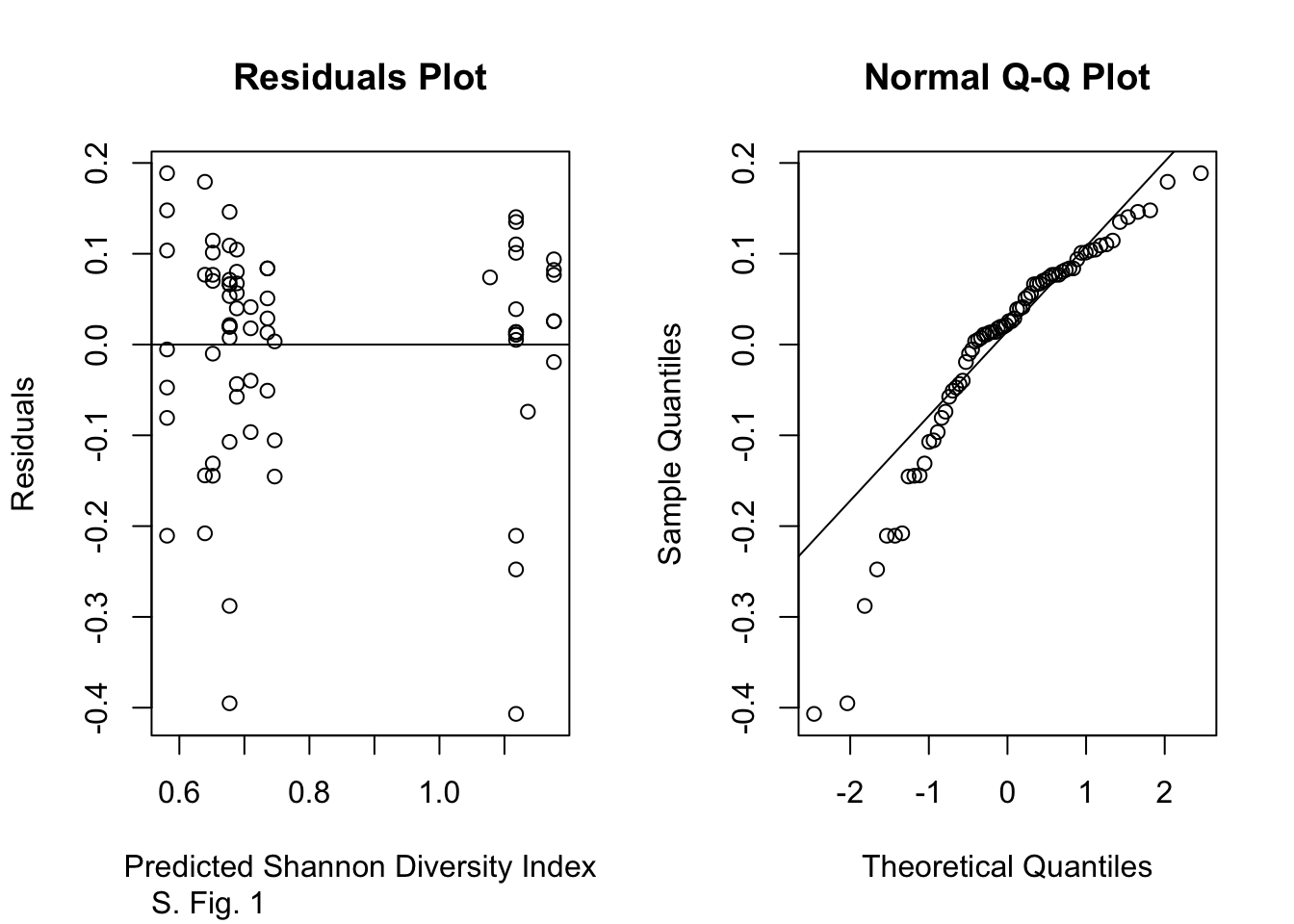

Code

# Histograms to visualize the distribution of the data
abundance_histogram <- ggplot(invert_data, 
                    aes(x = mean_org_per_plot)) +
  geom_histogram(fill = "lightgray",
                 col = "purple4") +
  theme_classic() +
  xlab("Mean Organisms per Plot")

shannon_histogram <- ggplot(invert_data, 
                    aes(x = shannon_index)) +
  geom_histogram(fill = "lightgray",
                 col = "purple4") +
  theme_classic() +
  xlab("Shannon Diversity Index")

histograms <- abundance_histogram + shannon_histogram

Code

histograms + plot_annotation(title = 'Histograms Showing Data Distribution')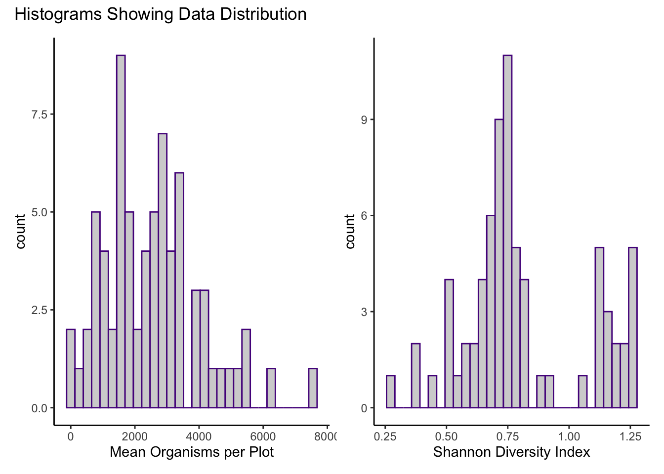

_S. Fig. 2

Code

# create data summary table

data_summary_table <- table(invert_data$intertidal_sitename, 
                            invert_data$drought_simple) 

kable(data_summary_table,
      col.names = c("Drought", "No Drought"),
      caption = "Sample size by site and drought condition.")

Sample size by site and drought condition.
	Drought	No Drought
Damnation Creek	3	7
Davenport Landing	1	1
Enderts	4	7
False Klamath Cove	4	7
Sandhill Bluff	6	13
Scott Creek	6	13

_{S. Table. 1}

References

1. Connell JH. The influence of interspecific competition and other factors on the distribution of the barnacle Chthamalus stellatus. Ecology (Durham). 1961;42(4):710–723. doi:10.2307/1933500

2. Paine RT. Marine rocky shores and community ecology: an experimentalist’s perspective. Oldendorf/Luhe, Germany: Ecology Institute; 1994. (Excellence in ecology, 4).

3. Tomanek L, Helmuth B. Physiological ecology of rocky intertidal organisms: a synergy of concepts. Integrative and Comparative Biology. 2002;42(4):771–775. doi:10.1093/icb/42.4.771

4. Denny M, Wethey D. Physical processes that generate patterns in marine communities | Denny Lab. 2001 [accessed 2022 Dec 2]. https://dennylab.stanford.edu/publications/physical-processes-generate patterns-marine-communities

5. Foster BA. Desiccation as a factor in the intertidal zonation of barnacles. Marine Biology. 1971;8(1):12–29. doi:10.1007/BF00349341

6. Menge BA, Lubchenco J, Bracken MES, Chan F, Foley MM, Freidenburg TL, Gaines SD, Hudson G, Krenz C, Leslie H, et al. Coastal oceanography sets the pace of rocky intertidal community dynamics. Proceedings of the National Academy of Sciences. 2003;100(21):12229–12234. doi:10.1073/pnas.1534875100

7. Helmuth B, Mieszkowska N, Moore P, Hawkins SJ. Living on the edge of two changing worlds: forecasting the responses of rocky intertidal ecosystems to climate change. Annual Review of Ecology, Evolution, and Systematics. 2006;37:373–404.

8. Cook BI, Mankin JS, Anchukaitis KJ. Climate change and drought: from past to future. Current Climate Change Reports. 2018;4(2):164–179. doi:10.1007/s40641-018-0093-2

9. Aspin TWH, Hart K, Khamis K, Milner AM, O’Callaghan MJ, Trimmer M, Wang Z, Williams GMD, Woodward G, Ledger ME. Drought intensification alters the composition, body size, and trophic structure of invertebrate assemblages in a stream mesocosm experiment. Freshwater Biology. 2019;64(4):750–760. doi:10.1111/fwb.13259

10. Fairbanks J, McArthur JV, Young CM, Rader RB. Consumption of terrestrial organic matter in the rocky intertidal zone along the central Oregon coast. Ecosphere. 2018 [accessed 2022 Nov 7];9(3). https://www.osti.gov/pages/biblio/1423921. doi:10.1002/ecs2.2138

11. Kautsky N. Quantitative studies on gonad cycle, fecundity, reproductive output and recruitment in a baltic Mytilus edulis population. Marine Biology. 1982;68(2):143–160. doi:10.1007/BF00397601

12. National Drought Mitigation Center (NDMC), the U.S. Department of Agriculture (USDA), the National Oceanic and Atmospheric Administration (NOAA). GIS Data | U.S. Drought Monitor. [accessed 2022 Dec 5]. https://droughtmonitor.unl.edu/DmData/GISData.aspx

13. Explore the Data | MARINe. MARINe | Multi-Agency Rocky Intertidal Network. [accessed 2022 Dec 5]. https://marine.ucsc.edu/explore-the-data/index.html

14. Engle JM, Anderson L, Burnaford JL, Douglas M, Lohse DP, Parsons-Field A. Unified monitoring protocols for the multi- agency rocky intertidal network. 2022. https://marine.ucsc.edu/longtermprotocol.pdf

15. US EPA. Ecoregions of North America. 2015 Nov 25 [accessed 2022 Dec 5]. https://www.epa.gov/eco-research/ecoregions-north-america

16. Bennett I, Pope EC. Intertidal zonation of the exposed rocky shores of Tasmania and its relationship with the rest of Australia. Marine and Freshwater Research. 1960;11(2):182–221. doi:10.1071/mf9600182

Citation

BibTeX citation:

@online{french2022,
  author = {Jessica French},
  title = {Drought {Impacts} on {Motile} {Invertebrates} in the {Rocky}
    {Intertidal}},
  date = {2022-12-07},
  url = {https://jessicafrench.github.io/2022-12-04-intertidal-iverts-drought/},
  langid = {en}
}

For attribution, please cite this work as:

Jessica French. 2022. “Drought Impacts on Motile Invertebrates in the Rocky Intertidal.” December 7, 2022. https://jessicafrench.github.io/2022-12-04-intertidal-iverts-drought/.